Excel is a requirement for most business jobs. Why wouldn’t it be? It’s a powerful tool for when it comes to dealing with lots of big data.

It can help organize data in a simple structure to most cases automatically. So why would anyone want to deal with that data manually? The ease of Excel is all you have to do is enter the formula and Viola! anything you would have had to do manually can be done automatically.

Need to display data in charts? do simple math? marge data? Excel can do it for you!

Chances are anytime you need to do a task that requires lots of manual labor, there is an excel formula for that.

Whether it’s for daily work, school project or personal use, to work more efficiently and avoiding manual work, mastering Excel is one skill you’d want to have.

Here are 10 useful Excel spreadsheet tips and tricks that may come in handy.

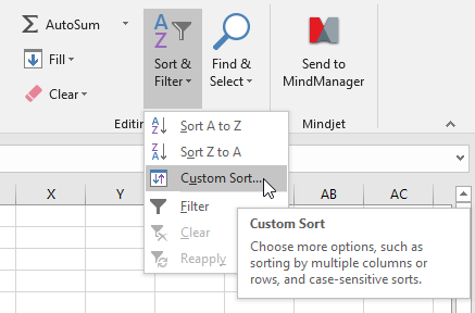
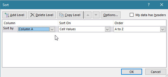
1. Custom sorting or filtering

Custom sorting can be used when a user is looking to filter or sort their current spread sheet based on multiple columns. For example, you may want to sort a spread sheet by first name, then last name, then date of birth.

To do so, start by highlight the excel sheet. Under the Home tab, click on the Sort & Filter icon on the top right side and select custom sort. A new dialog box will open — start with selecting the column to sort by first along with values to sort on and the order. Once complete, click add level to add additional levels of sorting. To finish, click OK and the sort order will be displayed.

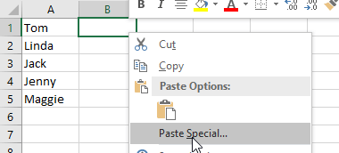
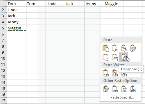
2. Transposing text

Transposing text can be used when you want to transform the cell items in rows into columns (or vice versa). Instead of copying and pasting individual rows or columns, use the transpose feature to move the row data into columns (or vice versa).

Select the column that you want to transpose into rows and copy (CTRL+ C). Select the row where you want to paste the data. Right-click on the first cell, and select Paste Special. A display box will appear — at the bottom, select the transpose option. Select OK to display your data. The same steps can be used when looking to transpose cell data from rows into columns.

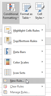
3. Conditional Formatting

Conditional formatting can be used to highlight any important information in your spreadsheet.

For example, if you keep a monthly expense sheet and want to see when you have exceeded a budgeted limit, you can format the cell to change colours when it’s close to your limit or has surpassed your limit.

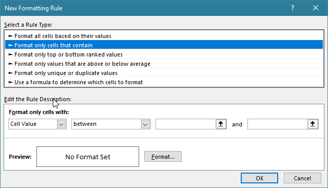
Select the cells you wish to conditional format. Under the Home tab, click Conditional Formatting and then New Rule. In the dialog box, click Format only cells that contain. In the Edit the Rule Description area, select Cell Value — greater than — insert the cell with the budgeted value. Once done, click OK to set the condition.

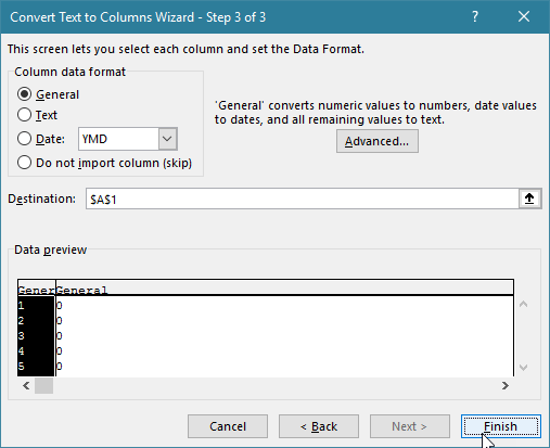
4. Text to Columns

Text to Columns can be used when you want to split the information in one cell into two different cells. For example, when you are looking to separate people’s full name into first and last name.

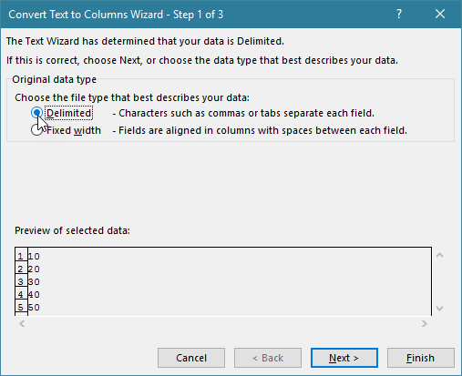
Start by highlight the column that you want to split. From the top navigation bar under the Data tab, select Text to Columns. A dialog box will appear.

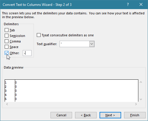
For the example above, you will want to select the Delimited option, which allows you to separate the information based on characters. Click Next to get to the following screen. Now select the Space option only and click Next. On the following keep the selection as General and hit Finish.

Note: You will want to have a few empty columns beside the selected column depending on the amount of information you are looking to split into individual cells.

5. Generating drop-down pick lists

Lists can be used to help speed up your work and add efficiency in your processes. Add a drop-down list for users to pick values from instead of adding them in.

In a column, type in the entries you wish to display as options of the pick list. Once done, select the range of cells you wish to have the pick list for. Under the Data tab, select Data Validation. Within the Settings tab, go to the Allowbox and select List from the menu. In the Source box, highlight the cell ranges that you typed your entries in for the list. Once done, click OK.

FORMULAS:

Photo by JESHOOTS.COM on Unsplash

6. Transforming the case of your text

These simple and easy to use formulas allow you to transform texts for different use cases. Use the UPPER formula to will capitalize all characters in a cell. Or, use the LOWER formula to change the text to all lower case letters in a cell. Use the PROPER formula to only only capitalize the first character of a word in a cell.

To copy these formulas to all cells in a column or row, simply drag the highlighted cell from the bottom right corner to all cells you wish to copy the formula to.

7. Count IF

This formula can be used to count the number of cells that fit a certain criteria.

For example to count the number of employees whose birthdays are in September, use the COUNTIF formula to say: =COUNTIF(“selected cell range that displays the birthday month”, “has the word September”).

8. IF Statements

IF statements come in handy when you are looking to make comparisons or run a logic test between a true value and a false value. The formula is used to say if a value is true, do X if not do Y.

For example, if you are looking to break up a group into two groups based on their age (Group A, age 1–25 and Group B, age 26–50), you can use the IF function to say: =IF(“selected cell range”<26, “Group A” (do X: assign to Group A), “Group B (if not do Y: assign to Group B).

9. Concatenate

This formula can be used to combine the values of selected cells into one. For Example, if you have a set of data that lists out first name and last name separately in two columns but you wish to have it in one, use the CONCATENATE formula to say: =CONCATENATE(“select cell range for first name”, “select cell range for last name”).

10. VLOOKUPS

VLOOKUPS are great when you have a large amount of data displayed in a table and you are looking to pull the information elsewhere on your spreadsheet. Instead of copying and pasting the data manually, use this function to make it automated.

For example, let’s say you have two sheets in sheet one is a criteria that reveals if your birthday is in September you get the number 9 assigned to you. In sheet two, you have a table with the a list of employees and their birthdays.

To assign the numbers from sheet one to sheet two, use the VLOOKUP formula to say: =VLOOKUP(“select cell range with the birth month of the employees in sheet two”, “select cell range that contains birth months in sheet one (range containing look up value), “select column that will contain the numerical value for the birthdays”, FALSE (for an exact match, can use TRUE for an approximate match).

Hopefully you found this helpful! Feel free to bookmark it to keep it handy and share any other handy Excel tips that you may have 🙂